The Velocity of Risk – What Bankers Need To Know

Banks that are looking to enhance their risk management practices should consider incorporating the concept of the velocity of risk into their enterprise-wide risk management practices. Some risks occur slowly; others strike quickly and hard. The velocity of risk is the time frame in which the risk may occur. In this age of social media, global interconnectedness, and market volatility, banks can be one tweet torrent away from a lightning-fast onset of risk. In this article, we explore why and how banks are starting to incorporate the “velocity of risk” into their risk management practices.

Optimizing Risk

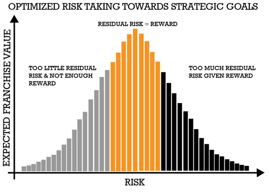
While we have discussed this framework before (HERE), it is our opinion that the goal of every banker is to optimize risk. After adjusting for mitigating factors, the residual risk falls on a spectrum, and banks need to ensure they are not taking too much or too little risk, given the reward. Banks that take too much risk fail, and banks that take too little risk produce returns below their cost of capital and either get acquired or driven out of business. This characteristic is why when you look at a graph of long-term bank performance, more banks underperform than overperform.

The Comparison of Risk

Currently, your bank measures the likelihood of a particular risk, the impact of that risk, the mitigation of that risk, and the expected quantification of that risk after the mitigating factors. However, that still does not put all risks on a level playing field.

Consider the risk above. One morning, President Trump tweeted his desire for an additional tax on all foreign-owned companies operating in the US. Instantly, the cash flow for those businesses that many community banks lent to is impacted. Valuations on those cash flows changed overnight, increasing a borrower’s probability of default and their loss given default. In this case, the expected loss changed by 30%. That is a significant change in risk for a material part of a large community bank’s balance sheet. Luckily, nothing became of it. Regardless, it was a risk that should have been accounted for nonetheless.

Now, there are the current high energy prices increasing the use of electric and hybrid vehicles. This has further hurt the cash flow at gas stations and convenience stores tied to gas stations. When this risk is quantified, it has changed the five-year expected loss outlook by a negative 30%.

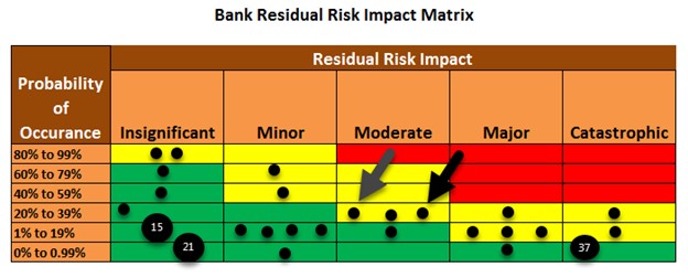
For some banks, the amount of gas station and convenience store loans is about equal to loans to US businesses that are owned by foreign nationals. Thus, the framework at most banks has these two risks as equal. This is diagramed below as the gray arrow, pointing to businesses that are foreign-owned, and the black arrow, pointing to c-store businesses, occupy the same risk category in the residual risk matrix.

 Speed Kills – The Velocity of Risk

However, the risk of these two events is not exactly equal. The first risk of a tax on foreign-owned companies resulted in an instantaneous credit shock, while the change in gas station demand will take place over years. This slower onset of risk will give banks time to adjust pricing, reduce exposure, and include additional risk mitigation mechanisms. That period of onset is known as the velocity of risk and measures the time between when the risk first appears and when it has a tangible impact on the bank.

The slower the velocity of risk, the more steps a bank can take in the post-event period to mitigate the risk impact and lower the residual risk. Conversely, the shorter the time, the fewer options a bank has, which lowers the chance of risk mitigation and increases an event’s residual risk.

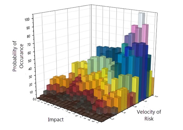
Similar to the probability of occurrence and the residual risk impact, the velocity of risk can be represented by banks by adding another dimension or axis to their risk map (below) so management can view all three dimensions.

Velocity and Residual Risk

Here is a crucial takeaway once you understand the velocity of risk – even if your bank is not going to incorporate the velocity of risk into its enterprise risk framework, it needs to take the velocity of risk into account when preplanning risk mitigation.  

We see all the time that a bank will include a mitigating factor to a specific risk so that the residual risk is negligible. Still, there is no way a bank can realistically carry out the mitigating factors in enough time for the mitigation to be effective. The result is an unrealistic view of risk that deceive both management and the regulators into believing the bank has a solid risk plan when in fact, they do not.

Examples abound, but a common one is when banks list “loan sales or participation” as a mitigant for credit shocks relating to lending sector concentrations. Back in September of 2007, when the first wave of credit shocks hit the market, banks had less than 45 days to unload their construction and raw land development (A&D) loans onto the market before it was common knowledge that the whole sector was toxic. Unfortunately, it takes about 60 days to sell a portfolio of loans, even for the most experienced bank.

No bank, to our knowledge, reacted fast enough, and by November of 2007, construction and development loans were trading at a 30% discount. At that point, banks were then reluctant to sell. By mid-2008, that turned into a 50% discount and then a 70% discount. The end effective result was that banks could not sell their exposure until the entire risk in the market materialized. The lesson is that there are few material mitigating factors to handle construction and development loan exposure post-credit shock.

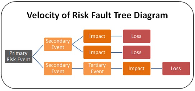
Measuring Velocity of Risk: The Fault Tree

Banks often map the velocity of risk through a fault tree analysis. By thinking through risk, practitioners can better understand the steps that risk would take as it flows from event to monetary loss. The more steps and the more time each step takes, the more risk a bank is exposed to when it comes to faster velocity events.

Back to our construction lending example – If it takes 60 days to sell a loan or to get the borrower to post additional collateral, then the bank is theoretically exposed to all relevant risks with a velocity of faster than 60 days. That means banks would have to analyze all post-event mitigating factors to ensure that they could execute in less than 60 days.

By diagraming out a fault tree, bankers can think through not only the primary event but second and tertiary events as well. For example, in Florida, we have a hurricane as a potential primary risk event, flooding as a secondary event, and then delays in clean-up as a tertiary event. The velocity of risk, in this case, is one to three days, with the impact most likely felt on day four and potential losses quantified in a period of several weeks. This time frame is slower than banks with lending exposure to earthquake risk but much faster than banks exposed to rising sea levels.

Using our hurricane example, banks can then use the fault tree to take steps to prepare for a hurricane, flooding, delays in emergency support, damage assessment, and restoration support. While mapping out a storm is straightforward, mapping out the velocity of risk for changes in a pandemic, alternative energy credits, or the impact of the Affordable Care Act changing is more complicated, which is all the more reason to try to understand those risks.

Quantifying The Velocity of Risk

While most banks will choose to subjectively quantify the velocity of risk into “Slow,” “Medium,” and “Fast” categories that align with “Low,” “Medium,” and “High” segments of other risk dimensions, we are fans of trying to quantify each category. We recommend measuring the velocity of risk by categorizing each risk into “Hours,” “Days,” “Months,” “Years,” and “Decades.” In this manner, you get more granularity, and you can also translate those labels into a mathematical formula for ranking residual risk.

Here are two methods of how incorporating the velocity of risk into a quantitative framework using a formula:

Simple: Risk = (Probability of risk event + Velocity) * Impact. Each risk factor is rated on a scale of one to five, with five being the highest probability, the fastest velocity (hours and days), and the greatest impact.

More Complex: Residual Risk = (Probability of risk event – probability of preventing risk event from impacting bank constrained by the velocity of risk) x (financial impact of risk event – financial mitigation)

For example, let’s go back to our convenience store (c-store) lending example. Assume a seven-year horizon that covers a five-year loan; we place the probability of having a credit event impacting the entire industry at close to 70%. As a result, we have increased our underwriting standards, tightened our loan structuring risk, and better segmented our pricing. Also, we have increased monitoring of all c-store loans.

We then access the velocity of risk. While the onset of consumer behavior will be slow, we are monitoring current gas prices and EV car/truck sales. Supply chain issues and rising costs have slowed this trend in recent months, thereby easing the rapid velocity of risk to this sector.

The Velocity of Risk Is Dynamic

Another critical concept to understand is that risk velocity is not static and is not a passive measure. Like other risk factors and mitigations, the velocity of risk can also be managed and controlled. Banks can do things to increase or decrease the velocity. In our hurricane example, while we cannot control the speed of when the hurricane hits, we can (and have) created a system to pick up hurricane formation earlier and then have developed a plan to communicate that information to all employees better. The net result is a decrease in the velocity of risk.

In our c-store example, an early warning system can be created by putting a line of credit in place or requiring data from the c-store’s point of sale system. A bank can gain better visibility when sales slow down. This can slow the velocity of risk by almost a year which is a significant improvement given how most banks now handle that risk. Slower velocity directly translates into better returns and/or lower capital allocation.

Putting Velocity of Risk into Action

In addition to training your bank staff on how to think about, discuss and manage the velocity of risks, banks would be well served to include velocity as another risk dimension in their framework. Banks should then size and quantify mitigating risk factors based on risk velocity to determine which can still apply to reduce risk and which are no longer valid. Then, banks should increase monitoring of those risk events that have high velocity. In some cases, this may mean putting additional risk controls in place, but often this means innovating new ways to control risk. Leveraging data, third-party monitoring, social media, sentiment analysis, or similar can all play a role in controlling the velocity of risk.

Factoring in the velocity of risk can apply to a complete risk category like credit or interest rate risk, or it can apply to a project or an operational risk such as the reliance on a fintech partner.

Risk management is still a relatively new discipline. Bankers need to continue to innovate and evolve their framework to improve as you update their strategic plan for next year or prioritize your current project initiatives list, factor in the risk of each project and what might keep you from achieving success. Factoring in the velocity of risk can help better rank and evaluate these efforts.

PWC published a four-page guide (HERE) for more information on the topic.

We are not sure there is anything more important than investing in risk management as it is the same economically as investing in revenue growth. Like credit, asset-liability management, and other banking functions, bankers need to consider a more holistic view and incorporate the new dimension of risk velocity.