Non-Maturity Deposits – A New Machined Learned Framework For ALM

Banking has now arrived at a speed that it cannot handle. While there have always been problems in banks’ asset-liability models (ALM) and liquidity stress test models, the current environment exacerbates this problem. Recent bank failures hurting public perceptions, the current market trends of higher rates, Quantitative Tightening, digital banking, social media, and a flight to safety have increased the difference between model and observed liability durations. As a result, most banks are overestimating their liability sensitivity and, thus, their deposit value. In this article, we will focus on non-maturity deposits to examine the problem and provide a solution.
Non-Maturity Deposit Background
Most all non-maturity deposits are lumped into a single category. Most banks think of this single category of non-maturity deposits, such as transaction accounts, as having a modified duration of about six. That is, for every increase in interest rates by 1%, the value of the liability increases by 6%. To calculate the duration of a liability product, you can observe how they have performed in the past.
Usually, banks look at their deposits and regress the deposit rates against the SOFR or a swap index. The output, or R-squared value, measures how much the change in SOFR can explain a deposit’s cost. In contrast to this deposit correlation, balances can be included in the calculation to correlate a deposit’s value to the SOFR or swap index. This is a bank’s deposit beta.
Banks often conduct a decay analysis to validate deposit assumptions. A static pool of deposits is analyzed to see how long they remain on a bank’s balance sheet over time. Banks take a pool from 2018 as an example and then track runoff to the present.
Utilizing this straightforward linear regression and decay analysis, you get something close to the profile below for the average community bank in the U.S.:
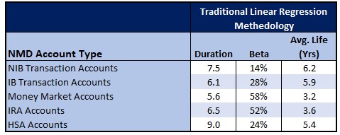
For most banks, the reality is that duration is much smaller, and the average life is a fraction of the traditional numbers.
The Challenge with Non-Maturity Deposit ALM Calculations
Unfortunately, several problems with the analysis lead to banks over-indexing on the stability and value of their non-maturity deposits. These problems are the following:
- Misunderstanding the nature of NMDs: NMDs are complex financial instruments that include embedded options for both the bank and customers. Banks have the option to adjust interest rates, while customers have the option to withdraw funds. Failing to understand and account for these options can lead to ineffective modeling and risk management.
- Inaccurate Options Value: When options value is modeled, they are usually modeled just for interest rate volatility. We are in a period of very high volatility, and the full impact of this optionality may not be correct. Further, the bank, and customer, have other, non-interest rate reasons for exercising their option, most notably safety. Usually, this helps reduce the value of the option to the customer (the option that the bank is short) and increase the value to the bank as community banks have historically been deemed safer than larger banks. Now, in this Too-Big-To-Fail environment, this is working against community banks, and the value of that option has increased. This reduces the duration of these non-maturity deposits.
- Inadequate Historical Balance Modeling: Relying solely on historical balance data is insufficient for NMD modeling, as it does not fully capture the dynamic nature of balance fluctuations. The increase in mobile and online banking, the inclusion of wires on these digital platforms, and the rise of social media have all served to speed up the potential for deposit outflows.
Prior to the failure of Silicon Valley Bank, the absolute worst-case scenario you could model was the Washington Mutual experience that had $8B, or 4% of their deposit base, leave the bank in three days utilizing 2,300 branches. Silicon Valley Bank presents a new high in lows with $42B, or 24% of liabilities. The bulk of these were non-maturity deposits, leaving the bank utilizing just 17 branches and their digital platforms in just over four hours. Had the bank opened the next day, it had outgoing wire orders for another $100B, totaling 81% of their deposit base.
Existing methodologies for non-maturity deposits now fail to model interest rate risk (IRR) accurately. As a result, institutions may encounter discrepancies between their model predictions and actual outcomes.
A New Methodology For ALM – Step 1: Forecasting The Environment
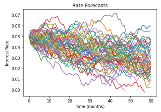
Instead of regressing deposit pricing and balances on a single metric, such as interest rates, the new “stochastic” approach utilizes a Monte Carlo term structure model to generate thousands of different environmental scenarios. To help us pull this off, we turn to Steven Wofford, CEO of the Kohl Analytics Group, to leverage their existing model.
Kohl’s term structure model is “calibrated” to historical rate movement. This ensures you are not looking at every potential scenario, only those where current rates, volatility, and means reversion probability would point to the highest probability of going over the next ten years. This limiting of potential rate movement allows for faster computations and gives banks a “probable worst case.” It is interesting to note that there are still many rate paths that go above 6% over the next five years.
Step 2: Forecasting Cashflows
Next, the model is trained to generate principal cashflows. The latest methodology is to use an unstructured machine-learned model. While many effective ways exist, one of the best methods is to use a “random forest” algorithm. This common algorithm combines the output of multiple decision trees to reach a single set of cashflows. One significant advantage is that the output is “explainable,” thereby limiting the “black box” syndrome of not knowing how the model generated the cashflows.
For Kohl analytics, some 20 or more variables are utilized, such as balance, account age, customer income, transaction history, customer age, account type, GDP, inflation, unemployment, and many other variables. Here, these variables can also be customized depending on the type of account. For health savings accounts, for example, the medical cost index can be included to improve forecast accuracy.
The model is then parameterized as you can tell the number of trees, the depth of each tree, and the fit of the model to the training data. The model is then run, evaluated, and refined by adding more variables or more parameters.
This method produces a non-maturity model baseline decay profile and creates alternative profiles at various levels. By synthesizing a decay stream algorithm under different rate scenarios, cashflows can be accurately and effectively managed.
Step 3: Adjust the Model For The New Environment
Once the base model is established, refinements take place to incorporate an “SVB Accelerator.” Here the size and percentage of uninsured deposits are added to the model. The amount of interest rate risk the bank AND borrower take is added to the model. Floating-rate loans or loans that are coming up for reset have higher probabilities of default. Conversely, fixed-rate loans that are “underwater” or have a below-market yield create additional risk for the bank. Unrealized bond losses are also included in the model.
Step 4: Combine Cashflows and Evaluate the Results
Principal and interest are then combined for each scenario. The scenarios are reduced to a single, probabilistic weighted cash flow that can be broken down by product, customer segment, customer persona, churn probability, or any number of different views. Banks can see a static and option-adjusted picture under various scenarios. For each view, banks can look at the duration, funds transfer pricing value, liquidity profile, and more.
Banks can also see cross-product value migration, such as when higher-priced money market accounts cannibalize savings and transaction accounts.
Finally, an economic value of equity (EVE) is calculated by deducting the variability of asset values minus the variability of liabilities, as is a market value added (MVA), which gets calculated by looking at the bank’s value less the amount of contributed equity capital. These calculations allow bankers to look at the return on assets and the return on equity for each instrument and customer segment.
How to Learn More About The Modern Forecasting of Non-Maturity Deposits
The reality is that banking has just evolved into more granularity and more accurate modeling of non-maturity deposits. Our industry can no longer be content with generic modeling of NMDs based on only historical rate movement. History is no longer a precursor to the future, and the world is more complicated than just worrying about interest rates alone. Being able to model various non-maturity products, uninsured deposits, customer segments, the propensity to use digital banking, and other several other dimensions against an array of variables will shortly become mandatory.
Suppose you want to learn more about how to adjust your asset-liability model and how to incorporate machine learning in the process. In that case, we have an upcoming webinar on the topic where we further explain this framework and show how most banks’ traditional linear regression framework overestimates the value, duration, and average life of non-maturity deposits by 2x or more. To learn more and to register, you can go HERE.